Reading and plotting data in Jupyter notebook

For this tutorial I am going to assume that you have some idea about using either Jupyter notebook or Python in general. I also assume that you have Anaconda installed, or know how to install packages into Python. If you do not, then I would first suggest putting a few minutes aside for installing Anaconda and taking a crash course in Jupyter.

The data structure

I am breaking down the data that I’m going to work with because the things I’m going to talk in this post can be applied to any other data which looks similar – That is, a simple two column data, which when plotted will form a 2D line plot with an x and y-axis.

In my lab we use a spectrometer to collect data. For the uninitiated, a spectrometer is basically a fancy prism with a camera at the rainbow end to take a black and white picture (intensity) of the rainbow. The data in this case is formed by spatially dispersing an input light into its constituent colors (wavelengths of that color). The intensity for each color is recorded using a camera. That is two columns of data – Wavelength is the first column, in nanometers and Intensity is the second column (photon counts, let’s say). The data file, of a near-infrared spectrum around 900 nm, if opened in a text editor, would look as follows.

900.0999819	1072801
900.200739	1087873
900.3014958	1101660
900.4022521	1113931
900.5030081	1118967
900.6037637	1099496
900.704519	1097624
900.8052738	1113681

If you would like to use the same data file I am using, you can download it from here.

Now, note that ASCII files like these are easier to handle for us starters and should show good numbers when opened using notepad or Microsoft excel.

Other proprietary formats such as the ones that directly come out of our spectrometer, like .SPE formats (for Princeton instruments cameras) is a binary format. These will give you garbage if you try to open these with notepad or excel. There is a way to open these using Python, but you need to have a detailed information about the format and construct the code accordingly to read them properly. In this post I’m going to deal with simpler ASCII (text, CSV files etc) files only.

If you are dealing with SPE or other such difficult file formats, I would suggest using a file conversion software that usually comes with the equipment to export the binary file to txt or csv format.

Importing libraries

Once you have the exported txt or csv, there’s a couple of ways to proceed. From my tests on time taken to read really large data files and for versatility (as you will see in the bonus tips), I have now settled on using pandas to read my files. This is a module that comes installed with Anaconda. Fire up your Jupyter notebook. To import this module you need to type in the following:

import pandas as pd

This imports the module pandas and all of the useful functions inside of it can be used using the “pd.” prefix. Similarly, the other scientific computing favorite, “numpy” is usually imported as “np” and you do it exactly what you did with pandas:

import numpy as np

Pandas is a great library for handling big datasets but we will use only a small part of it to read our data file. Numpy is a library that makes life easier when handling arrays, hence we import that too. We will see in the following code how these will be used. Running your code at this point will do nothing that you will see. You will certainly see errors if the modules were not installed properly.

Filename string

The most important thing you need to read a data file is its path – where is it in your computer? Say your file is in the same folder as your Jupyter notebook and is called “datafile.txt”. In this case you will first start by storing your file name in an arbitary variable, let’s say “filename”, like this:

filename = 'datafile.txt'

This stores the name of your file in the variable “filename”. And the type of this variable is string type – because it is text. This is the reason you need to put the quotations around the string when assigning it to the variable in the code.

But since files are not always conveniently inside the same folder as your code, you can also have the full path of the file stored in this string. This is always better. So now, say your file is in a folder ‘D:/data/datafile.txt’, then you store your full path+filename inside the filename variable as follows:

filename = 'D:/data/datafile.txt'

Read the file

To read the file using pandas now all you have to do is use the “read_csv” function from pandas as follows:

pd.read_csv(filename)

As long as you have a file with the column like data (shown previously) in it, you will immediately get a table as the output which for the type of data I showed above, would look like this:

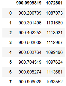
But this clearly is not desirable. Pandas read it all into a single column. To take care of that, we need to specify the delimiter to the read_csv function. The delimiter tells the function what separates your second column from your first column. In this case the delimiter is “\t” which is a string we use for tab in Python code. When it is separated by a space ” ” is the delimiter and when separated by commas, “,” is the delimiter and so on. The delimiter is specified using sep=”” in the read_csv function as follows:

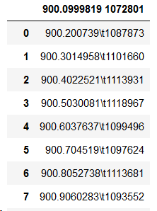
pd.read_csv(filename, sep='\t')

This gives an output which looks like this:

Which is also not very desirable because the two bold numbers on the top tell me that it read the first row of my data as a header, or the title of my columns. Pandas is a bit too smart to do that, because unlike usual data files we do not have column names in the first row of our file. It’s all data. We need to tell Pandas that by adding this specification. Here’s how you do it.

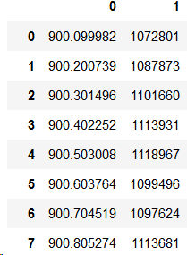
pd.read_csv(filename, sep='\t', header=None)

And that gives us a nice output which has several horizontal rows (only 8 rows shown here) and 2 vertical columns. Note that the header is simply indices now. The data is read inside the table.

I have figured that for simple data with two column of numbers, using pandas beyond this step is an overkill and requires you to learn several other smart quirks it has. Therefore I prefer storing all of the data retrieved by Pandas, in the form of bare-bone array of numbers. To do this you simply add “.values” to the end of your pandas read_csv function and store all of the numbers inside a variable called “data”. Here’s how:

data = pd.read_csv(filename, sep='\t', header=None).values

TLDR so far: In 3 lines of code and a few milliseconds of run time you get all of the data from your file! (we are not using the numpy import yet so that can be skipped). The final code we have now is:

import pandas as pd
filename = 'D:/data/datafile.txt'
data = pd.read_csv(filename, sep='\t', header=None).values

Working with the data – 2D array

The “data” variable now contains all the data from the filename. It is very convenient to access any part of the data or do math on it now.

Let’s say you need to get the x-axis column, i.e. the full first column of our file, into a variable called “x”. And let’s also do y-axis into a variable called “y” while we are at it. This can be done as follows:

x = data[:,0]
y = data[:,1]

Here the square brackets are used to access parts of an array. If we are dealing with a 2D array, like in the case of the “data” variable, we will need the row number and the column number of the data we want to access. These are put inside the square brackets where the first number represents the index of the row and second number is the index of the column, separated by a comma. In this case, since we want all the rows, the colon “:” gets all of the rows. Since x is the 0th index column (see the header in the data that was printed above), we tell the program to get all rows of 1st column (index 0) from the variable data by writing data[: , 0]. Similarly, all rows of 2nd column (index 1), by writing data[: , 1].

Fancier things can be done too. Like cutting and getting only a part of the data. Say you want all the x and y data from row 100 to row 200 (assuming you have that many rows), you can do this by writing:

x1 = data[100:200,0]
y1 = data[100:200,1]

Plotting your data

Plotting is most popularly and conveniently done using a library called matplotlib. Since we already have x and y arrays, both of same sizes taken out from our data file, this becomes very easy. First we import the plotting function we will need using the following:

import matplotlib.pyplot as plt

plt is a popular shortcut people use everywhere and that’s how I picked it up too. You may also use something of your own but it gets confusing fast. So I would suggest doing the same thing as everyone is doing. Same as pd for Pandas and np for numpy.

Now to plot we type in the following and run the cell.

plt.plot(x,y,'--')
plt.show()

The output for my data file shows as follows:

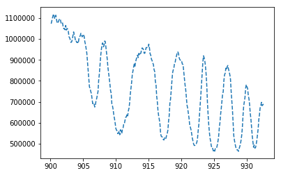
plt.plot(x,y) draws your line plot by taking the equal sized x and y arrays that we defined earlier. plt.scatter(x,y) can be used to make a scatter plot instead. While Python draws it in the background, it does not show it till you tell it to show what it drew. For that, we write the plt.show() part.

The color of the line, thickness, type of line, axis labels, text sizes etc can all be easily changed as per your liking. Refer to this documentation to do all of those things. And try making a green dashed line for your plot using plt.plot(x,y). Experiment by adding x and y labels to too.

TLDR: So now, the full code to import and plot in one place is as follows:

import pandas as pd
filename = 'D:/data/datafile.txt'
data = pd.read_csv(filename, sep='\t', header=None).values
x = data[:,0]
y = data[:,1]

import matplotlib.pyplot as plt
plt.plot(x,y)
plt.show()

Doing math on a data

Now let’s say you want to integrate the data from row 100 to row 200 (find area under the curve). For this the numpy we imported previously as np becomes useful. First we will define the part of the spectrum (x1 and y1) we want to integrate, if you haven’t done it previously.

import numpy as np
x1 = data[100:200,0]
y1 = data[100:200,1]
yint = np.trapz(x1,y1)
print(yint)

yint variable now contains is the integrated area under the part of the spectrum and is calculated using the trapezoidal method under numpy. More about it here. Printing out of the yint value gives you the integrated number value as the output.

To show the part of the spectrum we are integrating we can use axvspan and show it as follows. We first plot the full x and y columns using plt.plot(x,y), then use axvspan to show the range from x[100] to x[200], color it red and also make it half transparent by adding alpha = 0.5.

plt.plot(x,y)
plt.axvspan(x[100], x[200], color='red', alpha=0.5)
plt.show()

TLDR: So now, our full code to read the data, plot it, cut it, integrate and show the cut part of plot becomes:

%%time
import pandas as pd
import numpy as np
import matplotlib.pyplot as plt

filename = 'D:/data/datafile.txt'
data = pd.read_csv(filename, sep='\t', header=None).values
x = data[:,0]
y = data[:,1]
plt.plot(x,y)
plt.show()

x1 = data[100:200,0]
y1 = data[100:200,1]
yint = np.trapz(x1,y1)
print("Integrated area under the curve from",x[100],"to",x[200],"=", yint)
plt.plot(x,y)
plt.axvspan(x[100], x[200], color='red', alpha=0.5)
plt.show()

My output then looks like:

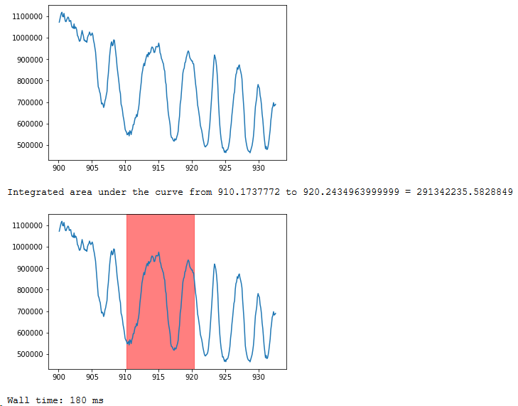
Bonus tips

Putting a magic command, “%%time” at the starting of the cell allows you to calculate the time taken to run the cell. In this case, all of this was done in 180 ms on my machine.

Not specifying a delimiter by saying sep=”none” and adding engine=’python’ in the pd.read_csv as follows, allows you to not specify any delimiter and read all ASCII files with ease. Pandas is smart enough to identify it on its own. I have tested this both with CSV (comma delimiter), space delimiter and tab delimiters. So now, the same line of code works with most of my data files!

data = pd.read_csv(filename, sep=None, header=None, engine='python').values

In case your file has header text in the first few lines, by saying header = None, you will be trying to read it in as data. You will end up getting garbage inside the variable data. To tackle this problem I would suggest adding skiprows=1, if you have one line of header text. Similarly, you would use skiprows=10 if you have 10 lines of header. In that case your code for pd.read_csv becomes:

data = pd.read_csv(filename, sep=None, header=None, engine='python', skiprows=1).values